Data format
Overview
The data format used in all scripts is based on the Astropy Table format. In the Build the
table section, we show how these Astropy Tables are created from the
DM butler. This work is automatically done for the deepCoadd_meas,
deepCoadd_forced_src, and forced_src catalogs, when avalaible,
and then saved together in one single hdf5
file. The procedure to write and read these files and work with the
loaded tables are described in the Working with the table section.
Build the table
The main table is built from the LSST DM butler as shown in the diagram [1] below:

For each filter f, an Astropy Table is created for all available
patches p1, p2, etc. Since we have the same number of patches
for all filters, which contain the exact same number of sources, all
table (1,p), (2,p), etc., created from a patch will be of the same
size for all filter. The Astropy Tables created from all individual
filters/patches set will then be vertically stacked. This means that if
we respectively have N1, N2 and N3 sources for the patches
1, 2 and 3, the output table will contains N1 + N2 + N3
sources. After the first stack, we end up with one table per filter,
all containing the same number of sources. These per-filter tables are
finally stacked together to form the final table shown on the
right-hand side of the diagram.
| [1] | Diagram created using https://www.jgraph.com/. Use the https://www.draw.io/?demo=1 application and the last xml file from this repository to update the diagram if needed. |
WCS
The WCS computed during the data processing is also stored in the
hdf5 file in the wcs path. If you load the data using the
read_hdf5 function, the
output will be a dictionary containing a wcs key, which refers to
an astropy.wcs.WCS
object. The skycoord_to_pixel and
pixel_to_skycoord
functions take this wcs object to convert the input coordinates
into an output format (sky <-> pixel).
All the tables (correspondig to the catalogs listed previously) already contain three coordinates columns:
coord_raandcoord_dec: they are the (ra, dec) coordinates in radian;coord_ra_degandcoord_dec: they are the (ra, dec) coordinates in degree;x_Srcandy_Src: they are the (x, y) position in pixel.
Working with the table
Note
The corresponding Jupyter notebook can be found here. You can also reproduce these results in ipython.
Astropy tables are great to work with, and can be used for all kind of
analysis in the context of our cluster study. You can apply filters,
group by column, concatenate them, etc. For a detailed review on
Astropy tables, see there.
Load the table
The Astropy tables created by the clusters_data step are saved
in an hdf5 file, and contains two main tables, corresponding to two
output catalogs of the data processing using the DM stack. As an
example, we will use here the deepCoadd_forced_src catalog, corresponding to the
forced photometry processing (some details).
If you want to start an analysis with an existing hdf5 file containing catalogs, you can use the one we have created for MACSJ2243.3-0935, which is saved at CC-IN2P3 under:
/sps/lsst/data/clusters/MACSJ2243.3-0935/analysis/output_v1/MACSJ2243.3-0935_data.hdf5
To load the deepCoadd_forced_src catalog, do:
from Clusters import data
f = "/sps/lsst/data/clusters/MACSJ2243.3-0935/analysis/output_v1/MACSJ2243.3-0935_data.hdf5"
d = data.read_hdf5(f)
fc = d['deepCoadd_forced_src']
d is a dictionnary containing the ‘deepCoadd_forced_src’, the ‘deepCoadd_meas’ catalogs and the ‘wcs’ object.
print d.keys()
['deepCoadd_forced_src', 'wcs', 'deepCoadd_meas']
and fc is an astropy table
print fc
base_CircularApertureFlux_3_0_flag_sincCoeffsTruncated ... coord_dec_deg
                                                       ...      deg
------------------------------------------------------ ... --------------
                                                 False ... -9.50417299504
                                                  True ... -9.50631091083
                                                  True ... -9.50631273401
                                                  True ... -9.50632589495
                                                  True ...  -9.5063327395
                                                 False ...  -9.5062460577
                                                  True ... -9.50629874096
                                                  True ... -9.50635437897
                                                 False ... -9.50600120865
                                                 False ... -9.50549567214
                                                   ... ...            ...
                                                 False ... -9.73333093082
                                                 False ... -9.73388006895
                                                 False ...  -9.7302761071
                                                 False ... -9.73010079525
                                                 False ... -9.72701283749
                                                 False ...  -9.7273114286
                                                 False ... -9.91085559972
                                                 False ... -9.91084514606
                                                 False ...  -9.8851539436
                                                 False ... -9.88578472829
Length = 1050500 rows
As you can see, there are
N = len(fc)
print N, "rows"
1050500 rows
in this table. This number correspond to the number of sources (ns) times the number of filters (nf): N = ns x nf. In this table, we have the following number of filter:
filters = set(fc['filter'])
nf = len(filters)
print nf, "filters:", filters
5 filters: set(['i', 'r', 'u', 'z', 'g'])
The number of sources in this catalog if thus:
ns = N / nf
print ns, "sources"
210100 sources
The number of columns corresponding to the number of keys available in the catalog is:
print "%i columns" % len(fc.keys())
for k in sorted(fc.keys())[:10]:
    print k
207 columns
base_CircularApertureFlux_12_0_flag
base_CircularApertureFlux_12_0_flag_apertureTruncated
base_CircularApertureFlux_12_0_flux
base_CircularApertureFlux_12_0_fluxSigma
base_CircularApertureFlux_12_0_mag
base_CircularApertureFlux_12_0_magSigma
base_CircularApertureFlux_17_0_flag
base_CircularApertureFlux_17_0_flag_apertureTruncated
base_CircularApertureFlux_17_0_flux
base_CircularApertureFlux_17_0_fluxSigma
Apply filters
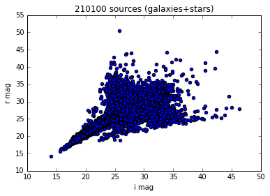
You can filter this table to, for example, only keep the i and r magnitude of the modelfit_CModel_mag for all sources:
magi = fc['modelfit_CModel_mag'][fc['filter'] == 'i']
magr = fc['modelfit_CModel_mag'][fc['filter'] == 'r']
and plot them against each other
# ignore the following line
%matplotlib inline
import pylab
pylab.scatter(magi, magr)
pylab.xlabel('i mag')
pylab.ylabel('r mag')
pylab.title('%i sources (galaxies+stars)' % len(magi))
<matplotlib.text.Text at 0x7f55453994d0>
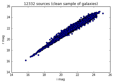
A few standard filters have been implemented in data and can be used directly to get a clean sample of galaxies:
# ignore the following line
import warnings; warnings.filterwarnings("ignore")
data_filtered = data.filter_table(d)
fc_filtered = data_filtered['deepCoadd_forced_src']
The same plot as in the above example now looks like
magi_filtered = fc_filtered['modelfit_CModel_mag'][fc_filtered['filter'] == 'i']
magr_filtered = fc_filtered['modelfit_CModel_mag'][fc_filtered['filter'] == 'r']
pylab.scatter(magi_filtered, magr_filtered)
pylab.xlabel('i mag')
pylab.ylabel('r mag')
pylab.title('%i sources (clean sample of galaxies)' % len(magi_filtered))
<matplotlib.text.Text at 0x7f55451f92d0>
See the code for a few other examples on how to use filters.
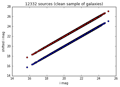
Add a new column
You can also add a new column to the table (examples here)
from astropy.table import Column
Create a simple shifted magnitude array
shifted_mags = fc_filtered['modelfit_CModel_mag'] + 2
Add it to the initial table and plot it against the initial magnitude (for the i filter here)
fc_filtered.add_column(Column(name='shifted_mag', data=shifted_mags,
                              description='Shifted magnitude', unit='mag'))
magi_filtered = fc_filtered['modelfit_CModel_mag'][fc_filtered['filter'] == 'i']
magi_shifted =  fc_filtered['shifted_mag'][fc_filtered['filter'] == 'i']
pylab.scatter(magi_filtered, magi_filtered)
pylab.scatter(magi_filtered, magi_shifted, c='r')
pylab.xlabel('i mag')
pylab.ylabel('shifted i mag')
pylab.title('%i sources (clean sample of galaxies)' % len(magi_filtered))
<matplotlib.text.Text at 0x7f55449552d0>
You can also add several columns using fc.add_columns([Columns(...), Columns(...), etc]).
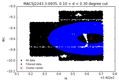
Filter around the cluster center
If you only want to work on a sample of galaxies center around the cluster at a certain radius, do:
confile = '/sps/lsst/data/clusters/MACSJ2243.3-0935/analysis/output_v1/MACSJ2243.3-0935.yaml'
config = data.load_config(confile)
output = data.filter_around(fc_filtered, config, exclude_outer=20, exclude_inner=3, unit='arcmin', plot=True)
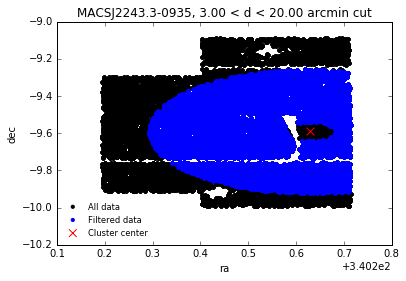
The output of filter_around is a filtered data table. You can also choose a different unit:
output = data.filter_around(fc_filtered, config, exclude_outer=0.3, exclude_inner=0.1, unit='degree', plot=True)